
Complete Guide to Pandas Datetime Operations: Master Time Series Data in Python (2025)
Working with time series data is one of the most critical skills for any data scientist or analyst. If you’ve ever struggled with date manipulation, timezone conversions, or time-based calculations in Python, you’re not alone. Fortunately, pandas datetime operations provide powerful tools to handle virtually any temporal data challenge you’ll encounter.
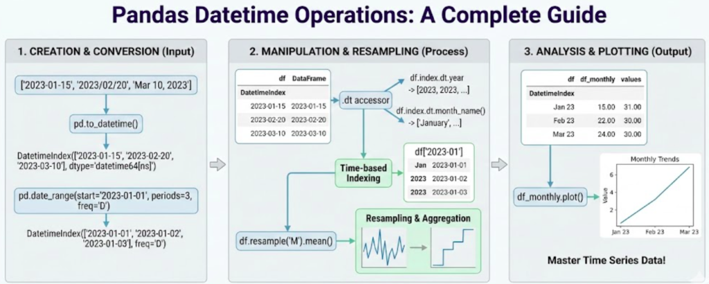
In this comprehensive guide, you’ll discover everything you need to know about pandas datetime operations, from basic date creation to advanced time series analysis. Whether you’re analyzing stock prices, weather data, or customer behavior patterns, mastering these techniques will transform how you work with temporal data.
What Are Pandas Datetime Operations?
Pandas datetime operations are specialized functions and methods designed to work with temporal data efficiently. The pandas library provides the pd.Timestamp class, DatetimeIndex, and the .dt accessor to manipulate dates, times, and timedeltas with ease.
🎯 Key Capabilities of Pandas Datetime Operations:
- Extract specific date components (year, month, day, hour)
- Perform date arithmetic and calculations
- Resample data to different time frequencies
- Handle timezone-aware datetime data
- Create sophisticated time-based analyses
- Generate business day calendars and custom periods
According to the official Pandas documentation, datetime functionality is one of pandas’ strongest features, making it the go-to library for time series analysis in Python.
Time series data appears everywhere in modern analytics: financial markets (stock prices, trading volumes), IoT sensors (temperature readings, motion detection), business metrics (sales data, user engagement), and scientific research (climate data, experimental measurements). Understanding pandas datetime operations allows you to extract actionable insights from these temporal datasets efficiently.
Creating DateTime Data in Pandas
The foundation of working with pandas datetime operations starts with creating datetime objects. Pandas offers several methods to generate date ranges and convert strings to datetime objects.
Using pd.date_range()
The pd.date_range() function is your primary tool for creating sequences of dates:
import pandas as pd
import numpy as np

# Create daily dates for an entire year
dates = pd.date_range(start='2025-01-01', end='2025-12-31', freq='D')
print(f"Generated {len(dates)} dates")

# Create hourly timestamps
hourly_data = pd.date_range('2025-01-01', periods=24, freq='h')

# Generate business days only
business_days = pd.date_range('2025-01-01', periods=20, freq='B')

# Create month-end dates
month_ends = pd.date_range('2025-01-01', periods=12, freq='ME')The freq parameter supports numerous frequency options including ‘D’ (daily), ‘h’ (hourly), ‘B’ (business days), ‘W’ (weekly), and ‘ME’ (month end). Check out Python’s datetime module documentation for more frequency codes.
Converting Strings to Datetime
When working with CSV files or databases, dates often come as strings. The pd.to_datetime() function handles conversion seamlessly:
# Convert string to datetime
date_string = '2025-01-15'
datetime_obj = pd.to_datetime(date_string)

# Handle multiple date formats
mixed_formats = ['2025-01-01', '01/15/2025', 'Jan 20, 2025']
parsed_dates = pd.to_datetime(mixed_formats, format='mixed')

# Convert entire DataFrame column
df['date_column'] = pd.to_datetime(df['date_column'])
These fundamental pandas datetime operations form the building blocks for all subsequent temporal data manipulation.
The .dt Accessor: Your Gateway to DateTime Properties
One of the most powerful features in pandas datetime operations is the .dt accessor. This special accessor provides access to datetime-specific properties and methods for Series objects.
Extracting Date Components
The .dt accessor makes it trivially easy to extract any component from datetime data:
# Create sample data
df = pd.DataFrame({
    'date': pd.date_range('2025-01-01', periods=100, freq='D'),
    'sales': np.random.randint(100, 1000, 100)
})

# Extract various components
df['year'] = df['date'].dt.year
df['month'] = df['date'].dt.month
df['day'] = df['date'].dt.day
df['day_of_week'] = df['date'].dt.dayofweek  # Monday=0
df['day_name'] = df['date'].dt.day_name()
df['month_name'] = df['date'].dt.month_name()
df['quarter'] = df['date'].dt.quarter
df['week'] = df['date'].dt.isocalendar().week

print(df.head(10))
Boolean Datetime Properties
The .dt accessor also provides boolean properties for common date checks:
# Check date properties
df['is_month_start'] = df['date'].dt.is_month_start
df['is_month_end'] = df['date'].dt.is_month_end
df['is_weekend'] = df['date'].dt.dayofweek.isin([5, 6])
df['is_quarter_start'] = df['date'].dt.is_quarter_startThese pandas datetime operations are incredibly useful for feature engineering in machine learning projects or for filtering data based on temporal conditions. Learn more about feature engineering techniques for time series on Kaggle.
Working with DateTime Index
Setting dates as your DataFrame index unlocks powerful time-based slicing and selection capabilities in pandas datetime operations.
Creating a DateTime Index
# Set datetime column as index
df_timeseries = df.set_index('date')

# Verify the index type
print(type(df_timeseries.index))  # DatetimeIndex
Partial String Indexing
One of the most convenient features of DatetimeIndex is partial string indexing:
# Select all data for a specific month
january_data = df_timeseries.loc['2025-01']

# Select a date range
date_range = df_timeseries.loc['2025-01-15':'2025-01-31']

# Select all data for a year
yearly_data = df_timeseries.loc['2025']
This intuitive syntax makes pandas datetime operations feel natural and readable, especially when exploring large time series datasets.
For learning Python data analysis comprehensively, I highly recommend Python for Data Analysis by Wes McKinney (Amazon affiliate link), written by the creator of pandas himself.
Resampling Time Series Data
Resampling is one of the most powerful pandas datetime operations for aggregating or disaggregating time series data to different frequencies.
Downsampling (Aggregating to Lower Frequency)
Downsampling combines multiple observations into fewer, lower-frequency observations:
# Create hourly data
hourly_data = pd.DataFrame({
    'timestamp': pd.date_range('2025-01-01', periods=168, freq='h'),
    'temperature': np.random.randint(20, 35, 168),
    'humidity': np.random.randint(40, 80, 168)
}).set_index('timestamp')

# Resample to daily averages
daily_avg = hourly_data.resample('D').mean()

# Multiple aggregations
daily_stats = hourly_data.resample('D').agg({
    'temperature': ['mean', 'min', 'max'],
    'humidity': ['mean', 'std']
})

print(daily_stats.head())
Upsampling (Disaggregating to Higher Frequency)
Upsampling creates more frequent observations from less frequent data:
# Daily data
daily_data = pd.DataFrame({
    'date': pd.date_range('2025-01-01', periods=7, freq='D'),
    'value': [100, 150, 120, 180, 200, 160, 190]
}).set_index('date')

# Upsample to 6-hourly with forward fill
hourly_data = daily_data.resample('6h').ffill()

# Upsample with interpolation
hourly_interpolated = daily_data.resample('6h').interpolate()
Custom Resampling Rules
Pandas datetime operations allow flexible custom aggregation logic:
# Weekly aggregation with custom rules
weekly_summary = df_timeseries.resample('W').agg({
    'sales': ['sum', 'mean', 'std'],
    'quantity': 'sum',
    'customers': 'nunique'
})
These resampling capabilities are essential for time series forecasting and analysis workflows.
Handling Time Zones Like a Pro
Global data analysis requires proper timezone handling. Pandas datetime operations provide comprehensive timezone support through the pytz library.
Timezone Localization
Convert timezone-naive datetime to timezone-aware:
# Create naive datetime
naive_dates = pd.date_range('2025-01-01', periods=5, freq='D')

# Localize to specific timezone
utc_dates = naive_dates.tz_localize('UTC')
print(utc_dates)

# Create timezone-aware range directly
aware_range = pd.date_range('2025-01-01', periods=24, freq='h', tz='UTC')
Timezone Conversion
Convert between different timezones:
# Convert UTC to other timezones
ny_time = utc_dates.tz_convert('America/New_York')
tokyo_time = utc_dates.tz_convert('Asia/Tokyo')
london_time = utc_dates.tz_convert('Europe/London')

# In DataFrames
df['timestamp_utc'] = pd.to_datetime(df['timestamp']).dt.tz_localize('UTC')
df['timestamp_local'] = df['timestamp_utc'].dt.tz_convert('America/Los_Angeles')Always store datetime data in UTC in databases and convert to local timezones only for display purposes. This prevents numerous timezone-related bugs. For more information about timezone best practices, check out Python’s timezone documentation.
Date Offsets and Business Days
Pandas datetime operations include sophisticated date offset objects for business logic and calendar arithmetic.
Basic Date Offsets
from pandas.tseries.offsets import BDay, MonthEnd, Week, Hour, Day

start_date = pd.Timestamp('2025-01-01')

# Add business days
next_bday = start_date + 5 * BDay()

# Move to month end
month_end = start_date + MonthEnd()

# Add weeks
two_weeks_later = start_date + 2 * Week()

# Combine offsets
complex_offset = start_date + 10 * BDay() + 3 * Hour()
Custom Business Day Calendars
Create custom business day calendars excluding holidays:
from pandas.tseries.offsets import CustomBusinessDay

# Define holidays
us_holidays = [
    '2025-01-01',  # New Year
    '2025-07-04',  # Independence Day
    '2025-12-25',  # Christmas
]

# Create custom business day calendar
us_bd = CustomBusinessDay(holidays=us_holidays)

# Generate business day range
business_dates = pd.bdate_range('2025-01-01', '2025-12-31', freq=us_bd)
print(f"Business days in 2025: {len(business_dates)}")
These pandas datetime operations are crucial for financial analysis, where business day calculations must exclude weekends and holidays.
Time Deltas and Duration Calculations
Calculating durations and time differences is a common requirement in pandas datetime operations.
Basic Time Delta Operations
# Create sample event data
df_events = pd.DataFrame({
    'start': pd.to_datetime(['2025-01-01 10:00', '2025-01-01 14:00']),
    'end': pd.to_datetime(['2025-01-01 12:30', '2025-01-01 15:45'])
})

# Calculate duration
df_events['duration'] = df_events['end'] - df_events['start']

# Convert to hours and minutes
df_events['hours'] = df_events['duration'].dt.total_seconds() / 3600
df_events['minutes'] = df_events['duration'].dt.total_seconds() / 60

print(df_events)
Date Arithmetic
# Add timedelta to dates
df['delivery_date'] = df['order_date'] + pd.Timedelta(days=7)
df['reminder_date'] = df['event_date'] - pd.Timedelta(hours=24)

# Calculate age or days since
df['days_since_signup'] = (pd.Timestamp.now() - df['signup_date']).dt.days
Rolling Windows for Time Series
Rolling window calculations are essential pandas datetime operations for smoothing data and identifying trends.
Fixed Window Rolling
# Create time series data
df_ts = pd.DataFrame({
    'date': pd.date_range('2025-01-01', periods=365, freq='D'),
    'value': np.random.randn(365).cumsum() + 100
}).set_index('date')

# Calculate rolling averages
df_ts['MA_7'] = df_ts['value'].rolling(window=7).mean()
df_ts['MA_30'] = df_ts['value'].rolling(window=30).mean()

# Rolling standard deviation
df_ts['volatility'] = df_ts['value'].rolling(window=20).std()
Time-Based Rolling Windows
Unlike fixed-window rolling, time-based windows consider actual time periods:
# Rolling window based on time period (not row count)
df_ts['rolling_7d'] = df_ts['value'].rolling('7D').mean()
df_ts['rolling_30d'] = df_ts['value'].rolling('30D').mean()

# Useful for irregular time series
irregular_data = df_ts.resample('3D').mean()
irregular_data['rolling_avg'] = irregular_data['value'].rolling('14D').mean()
Exponential Weighted Moving Average
# EWMA gives more weight to recent observations
df_ts['ewma'] = df_ts['value'].ewm(span=14).mean()
df_ts['ewm_std'] = df_ts['value'].ewm(span=14).std()
Pandas datetime operations like rolling windows are fundamental for technical analysis in trading strategies.
Advanced Time Series Analysis
Let’s explore sophisticated pandas datetime operations for comprehensive time series analysis.
Calculating Returns and Changes
# Percentage change
df_ts['pct_change'] = df_ts['value'].pct_change() * 100

# Absolute change
df_ts['abs_change'] = df_ts['value'].diff()

# Cumulative sum
df_ts['cumsum'] = df_ts['value'].cumsum()

# Cumulative product (compound returns)
df_ts['cum_returns'] = (1 + df_ts['pct_change']/100).cumprod()
Lag and Lead Operations
# Create lagged features
df_ts['lag_1'] = df_ts['value'].shift(1)
df_ts['lag_7'] = df_ts['value'].shift(7)

# Lead values
df_ts['lead_1'] = df_ts['value'].shift(-1)

# Calculate with lagged values
df_ts['change_from_week_ago'] = df_ts['value'] - df_ts['lag_7']
Seasonal Decomposition
# Group by season
df_ts['month'] = df_ts.index.month
monthly_avg = df_ts.groupby('month')['value'].mean()

# Day of week patterns
df_ts['day_of_week'] = df_ts.index.dayofweek
weekly_pattern = df_ts.groupby('day_of_week')['value'].mean()
For deep learning on time series, explore TensorFlow’s time series tutorials.
Common Pitfalls and Best Practices
Mastering pandas datetime operations also means avoiding common mistakes:
✅ Best Practices Checklist:
- Always Use Timezone-Aware Datetime: Use
.dt.tz_localize('UTC')instead of naive datetime - Set Datetime as Index: Enables powerful time-based operations for time series data
- Use .loc[] for Partial String Indexing: Correct way to slice by date strings
- Handle Missing Dates Explicitly: Use
.asfreq()with forward fill or interpolation - Vectorize DateTime Operations: Use
.dtaccessor instead of iterating through rows
Vectorized pandas datetime operations using the .dt accessor are 100-1000x faster than iterative approaches. Always prefer vectorization over loops when working with datetime data.
Frequently Asked Questions
pd.to_datetime() function: df['date'] = pd.to_datetime(df['date_string']). For mixed formats, use format='mixed' parameter..dt.tz_localize() to add timezone information to naive datetime, and .dt.tz_convert() to convert between different timezones.CustomBusinessDay from pandas.tseries.offsets to create custom calendars excluding specific holidays and weekends for business day calculations..asfreq() to establish regular frequency, then apply .ffill() (forward fill), .bfill() (backward fill), or .interpolate() to fill missing values..dt.days, .dt.seconds, or .dt.total_seconds() to extract the difference in desired units.df['year'] = df['date'].dt.year. This is orders of magnitude faster than iterating through rows.Conclusion
Mastering pandas datetime operations is essential for any data professional working with time series data. From basic date creation and the versatile .dt accessor to advanced resampling and rolling window calculations, pandas provides comprehensive tools for temporal data analysis.
🎓 Key Takeaways:
- Use
pd.date_range()andpd.to_datetime()for creating and parsing dates - Leverage the
.dtaccessor for extracting datetime components efficiently - Set datetime as your index for powerful time-based slicing capabilities
- Master resampling for aggregating data to different frequencies
- Handle timezones properly to avoid bugs in global applications
- Apply rolling windows and time deltas for sophisticated analysis
By implementing these pandas datetime operations in your workflow, you’ll handle time series data with confidence and efficiency. Whether you’re analyzing financial markets, IoT sensor data, or business metrics, these techniques form the foundation of professional-grade temporal data analysis.
🚀 Ready to Level Up Your Pandas Skills?
Continue your pandas journey and master data analysis with these comprehensive resources!
Explore More Tutorials